ECG Data Compression

In this example, we demonstrate the compression of ECG data using biorthogonal wavelets. We shall first go through different steps of the wavelet compression algorithm one by one. We will then show a unified encoder decoder function.

This example is adapted from the sample code provided in nerajbobra/wavelet-based-ecg-compression. Do refer to its documentation to get a general sense of the compression algorithm.

This implementation is significantly different and optimized.

# Configure JAX to work with 64-bit floating point precision.
from jax.config import config
config.update("jax_enable_x64", True)

Let’s import necessary libraries

import jax
import numpy as np
import jax.numpy as jnp
# CR-Suite libraries
import cr.nimble as crn
import cr.nimble.dsp as crdsp
import cr.wavelets as crwt
from cr.wavelets.codec import *
from cr.wavelets.plots import *
# Sample data
from scipy.misc import electrocardiogram
# Plotting
import matplotlib.pyplot as plt
# Miscellaneous
from scipy.signal import detrend

Encoder Configuration

# Number of samples per signal
NUM_SAMPLES_BLOCK = 3000
# Name of wavelet to be used for signal decomposition
WAVELET_NAME = 'bior4.4'
# Number of levels of decomposition
WAVELET_LEVEL = 5
# Fraction of energy to be preserved in each decomposition level
WAVELET_ENERGY_THRESHOLDS = [0.999, 0.97, 0.85, 0.85, 0.85, 0.85]
# Maximum percentage root mean square difference acceptable in quantization
MAX_PRD = 40 # percent

Test signal

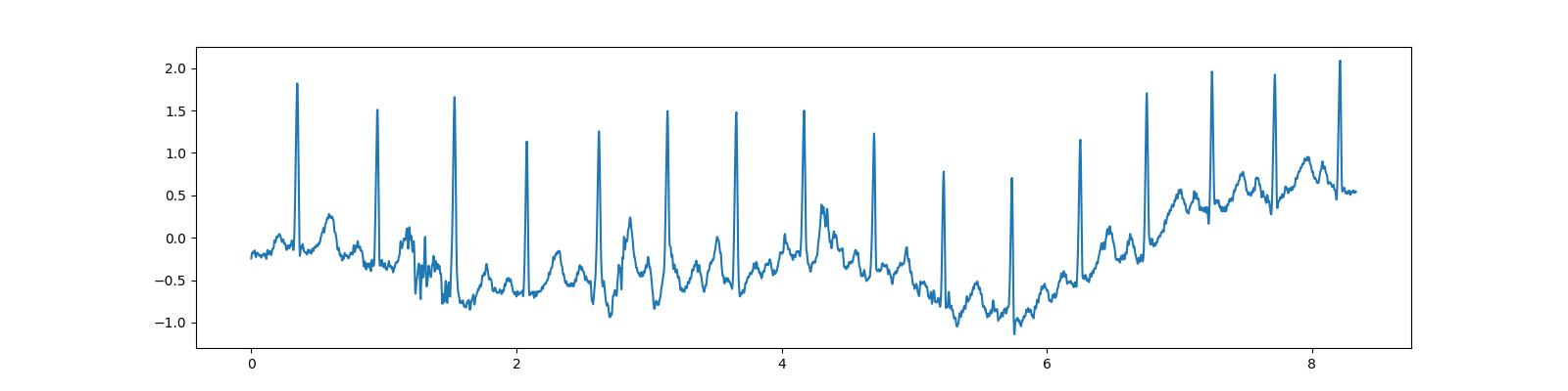
SciPy includes a test electrocardiogram signal which is a 5 minute long electrocardiogram (ECG), a medical recording of the electrical activity of the heart, sampled at 360 Hz.

ecg = electrocardiogram()
# Sampling frequency in Hz
fs = 360
# We shall only process one signal in this demo
signal = ecg[:NUM_SAMPLES_BLOCK]
n = len(signal)
t = np.arange(n) * (1/fs)
fig, ax = plt.subplots(figsize=(16,4))
ax.plot(t, signal);

/home/docs/checkouts/readthedocs.org/user_builds/cr-wavelets/checkouts/stable/examples/ecg_compression.py:70: DeprecationWarning: scipy.misc.electrocardiogram has been deprecated in SciPy v1.10.0; and will be completely removed in SciPy v1.12.0. Dataset methods have moved into the scipy.datasets module. Use scipy.datasets.electrocardiogram instead.
  ecg = electrocardiogram()

[<matplotlib.lines.Line2D object at 0x7f5f41be8760>]

Preprocessing

# Remove the linear trend from the signal
signal = detrend(signal)
fig, ax = plt.subplots(figsize=(16,4))
ax.plot(t, signal);

[<matplotlib.lines.Line2D object at 0x7f5f41f35f10>]

Encoder

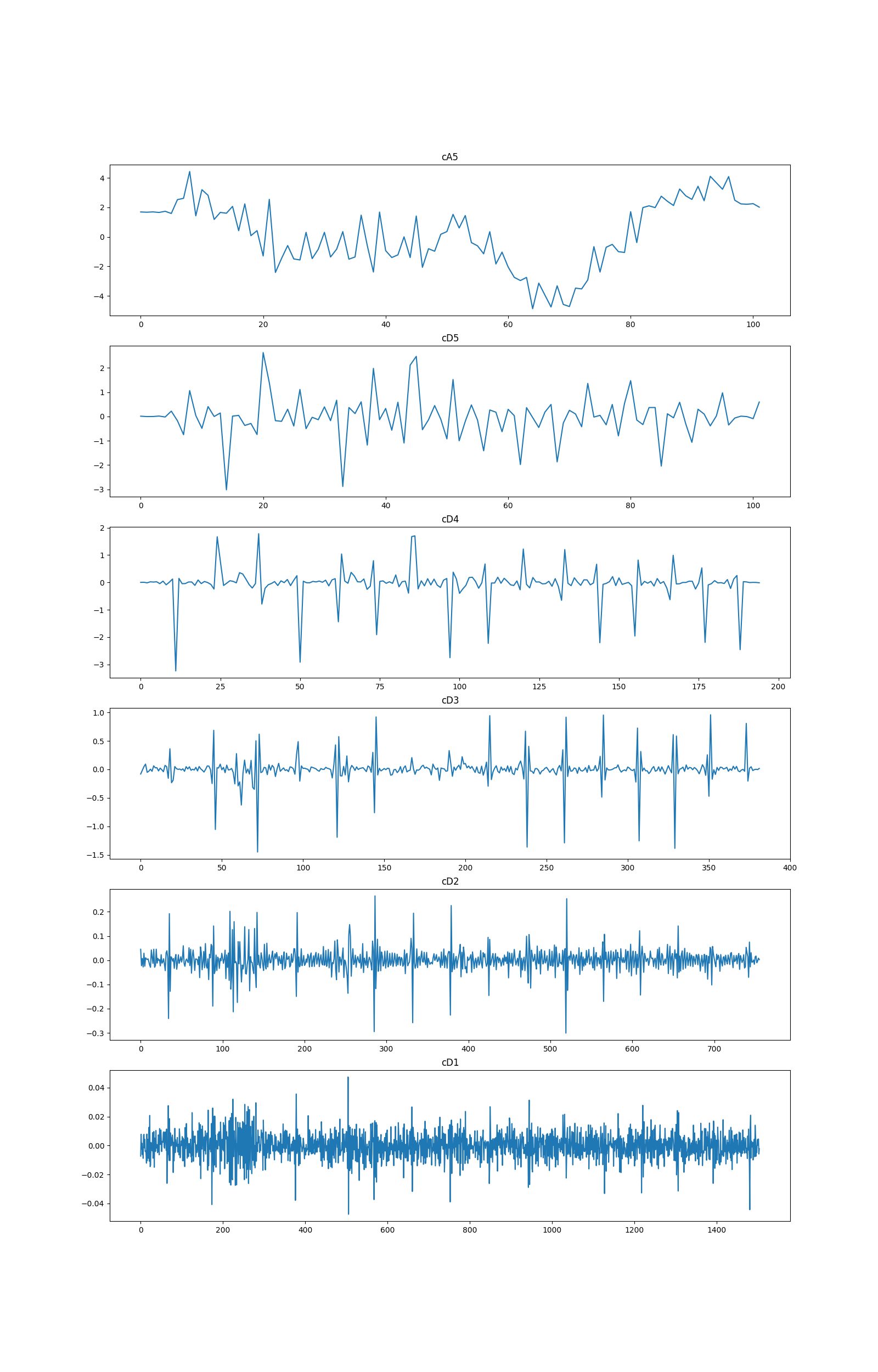
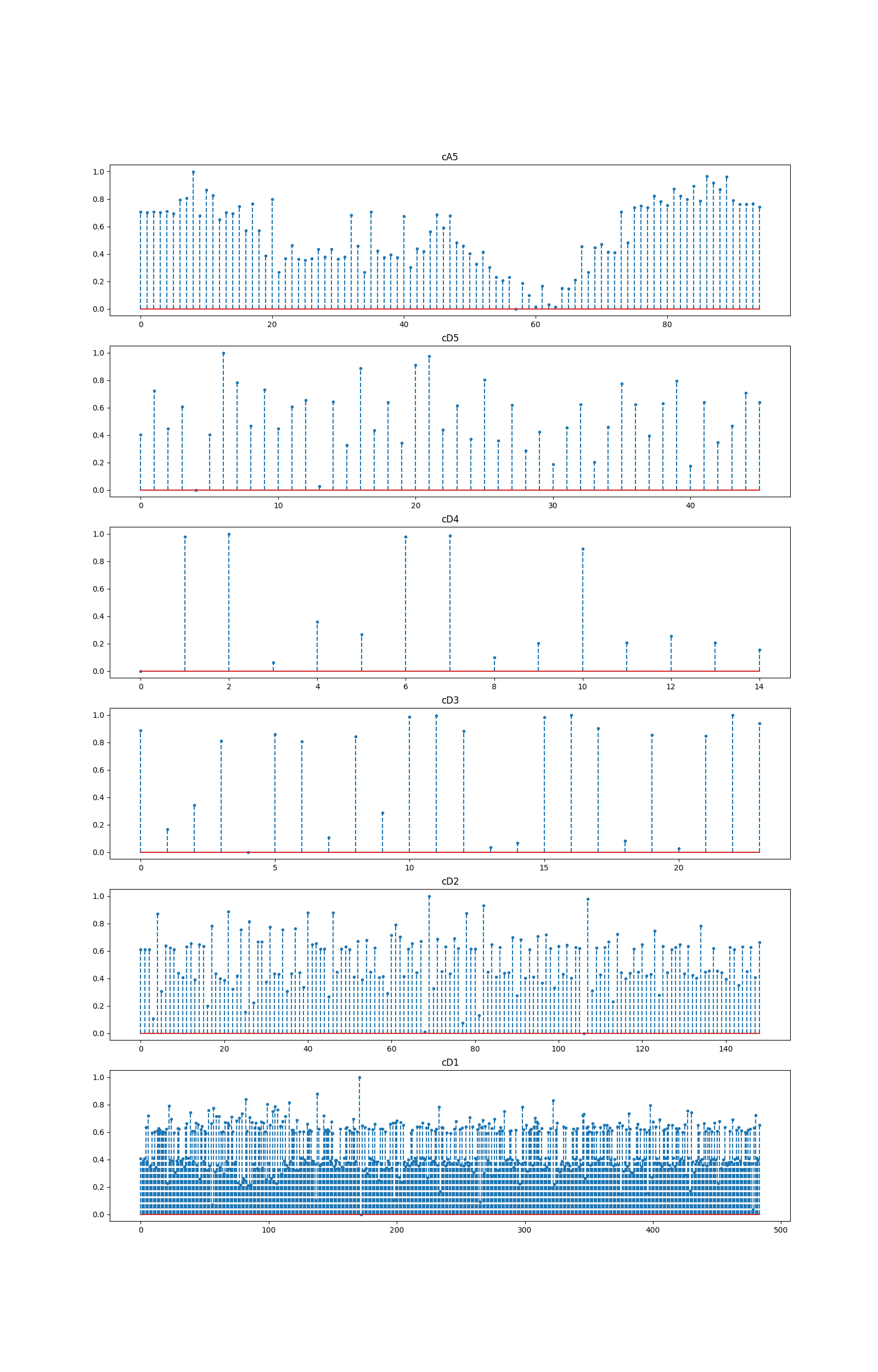
Let us perform a wavelet decomposition of this signal

wavelet = crwt.to_wavelet(WAVELET_NAME)
coeffs = crwt.wavedec(signal, wavelet, level=WAVELET_LEVEL)
fig, axes = plt.subplots(6, 1, figsize=(16,25))
plot_decomposition(fig, axes, coeffs)

Let us check the quality of the reconstruction

rec = crwt.waverec(coeffs, wavelet)
fig, ax = plt.subplots(figsize=(16,5))
plot_2_signals(fig, ax, signal, rec, fs=fs)

Percentage root mean square difference

print(crn.prd(signal, rec))

1.0158245596205641e-05

Let us threshold different levels of decomposition by keeping as few large coefficients as required to meet the target energy fraction (separately for each level)

th_coeffs, binmaps = threshold(coeffs, WAVELET_ENERGY_THRESHOLDS)
# Let us plot them to see the coefficients which have been zeroed out
fig, axes = plt.subplots(6, 1, figsize=(16,25))
plot_2_decompositions(fig, axes, coeffs, th_coeffs, label2='Thresholded')

Let us remove the zero entries from thresholded coefficients

nz_th_coeffs = remove_zeros(th_coeffs, binmaps)
# number of non-zero coefficients left at each level
for c in nz_th_coeffs: print(len(c))

95
46
15
24
149
484

Let us check how much loss we have suffered due to thresholding

# Add back the zeros
tmp = add_zeros(nz_th_coeffs, binmaps)
# Perform reconstruction using thresholded coefficients
th_rec = crwt.waverec(tmp, wavelet)
fig, ax = plt.subplots(figsize=(16,5))
plot_2_signals(fig, ax, signal, th_rec, fs=fs)
# Compute the percentage root mean square difference
print(crn.prd(signal, th_rec))

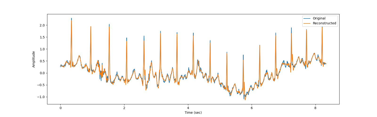
16.568432073643812

Let us now scale the nonzero thresholded coefficients to 0-1 range

scaled_coeffs, shifts, scales = scale_to_0_1(nz_th_coeffs)
# Let us plot to verify that they are indeed now in 0-1 range
fig, axes = plt.subplots(6, 1, figsize=(16,25))
plot_decomposition(fig, axes, scaled_coeffs, stem=True)

Let us quantize the scaled coefficients so that we meet the maximum PRD criteria.

(quantized_coeffs, num_bits,
    cur_prd) = quantize_to_prd_target(signal,
    WAVELET_NAME, WAVELET_LEVEL,
    scaled_coeffs, shifts, scales, binmaps, MAX_PRD)
# Let us look at the quantized coefficients at each decomposition level
fig, axes = plt.subplots(6, 1, figsize=(16,25))
plot_decomposition(fig, axes, quantized_coeffs, stem=True)
# Check how many bits are being used per sample and the achieved PRD
print(num_bits, cur_prd)

4 18.17883530994624

Merge the coefficients and binary maps of different levels to single arrays

combined_coeffs = combine_arrays(quantized_coeffs)
combined_binmaps = combine_arrays(binmaps)
print(len(combined_coeffs), len(combined_binmaps))

813 3041

We are now ready with all the data that needs to be transmitted to the decoder. This includes:

• The quantized nonzero coefficients

• The binary maps

• The shifts and scales for each level used during scaling

• The number of bits per sample used for quantization

We shall use the coding function which will compress all of this data into a packed bitarray.

result = encode_cbss_to_bits(combined_coeffs, combined_binmaps,
    shifts, scales, num_bits)

Check the number of bits used in compressing the whole block

print(len(result))

7108

We can also check the average number of bits per sample

print(len(result)/NUM_SAMPLES_BLOCK)

2.3693333333333335

The MIT-BIH database is encoded at 11-bits per sample. We can use this to compute the compression ratio

compression_ratio = len(signal) * 11 / len(result)
print(compression_ratio)

4.642656162070906

Decoding

We note that the decoder has access to only the encoded bitstream and the encoder configuration parameters. It doesn’t have access to any other intermediate data that was produced during encoding.

The first step is to extract all the data from the packed bitarray. Note that the number of bits per sample used for quantization is also being read from the bitstream.

(dec_c_coeffs, dec_c_binmaps,
 dec_shifts, dec_scales, dec_qbits) = decode_cbss_from_bits(
    WAVELET_NAME, WAVELET_LEVEL, NUM_SAMPLES_BLOCK, result)
# Since we have encoding steps data available, we can
# cross check to see if the data extraction from the
# bitstream happened correctly.
print(np.allclose(shifts, dec_shifts))
print(np.allclose(scales, dec_scales))
print(np.allclose(combined_binmaps, dec_c_binmaps))
print(np.allclose(combined_coeffs, dec_c_coeffs))

True
True
True
True

Let us now split the coefficients and binary maps to different decomposition levels

dec_coeffs, dec_binmaps = split_coefs_binmaps(
    WAVELET_NAME, WAVELET_LEVEL, NUM_SAMPLES_BLOCK,
    dec_c_coeffs, dec_c_binmaps)

Perform inverse quantization of nonzero coefficients

inv_quant_coeffs = inv_quantize_1(dec_coeffs, dec_qbits)

Perform descaling of the coefficients from [0, 1] range to their original ranges

dec_unscaled_coeffs = descale_from_0_1(inv_quant_coeffs, dec_shifts, dec_scales)

Add back the zero entries using the binary maps

dec_coeffs = add_zeros(dec_unscaled_coeffs, dec_binmaps)

Perform reconstruction of the signal from the decoded wavelet decomposition

dec_reconstructed = crwt.waverec(dec_coeffs, wavelet)
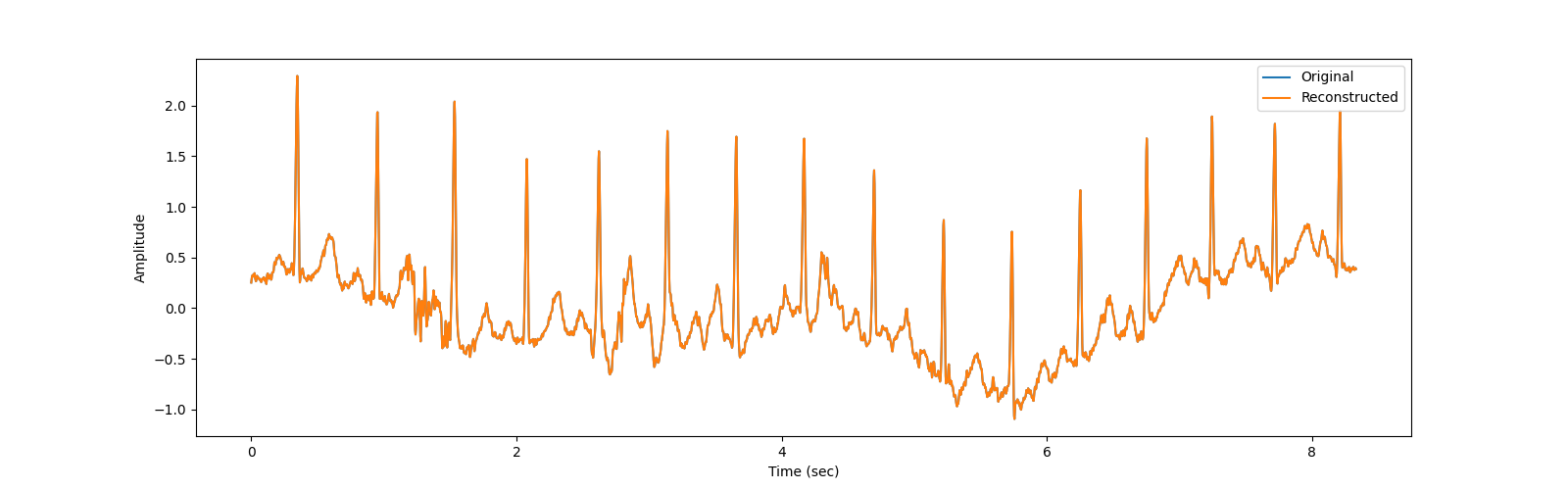
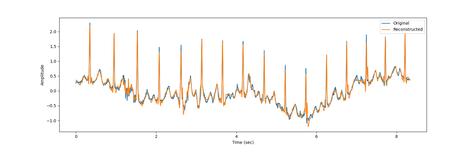
# Plot the original signal and reconstructed signal together
fig, ax = plt.subplots(figsize=(16,5))
plot_2_signals(fig, ax, signal, dec_reconstructed, fs=fs)

Measure the percentage root mean square difference

print(crn.prd(signal, dec_reconstructed))

18.178835029200155

Full CODEC

Carefully carrying out individual steps in the compression and reconstruction is hard. It would be great if the library can provide simple functions which wrap all the encoding and decoding operations together.

We can use the build_codec function to build an encoder and decoder function based on the encoder configuration parameters

encoder, decoder = build_codec(
    WAVELET_NAME, WAVELET_LEVEL, NUM_SAMPLES_BLOCK, MAX_PRD, WAVELET_ENERGY_THRESHOLDS)

Let us use the encoder to compress the signal

bits = encoder(signal)

Check that the encoder function did exactly the same thing as our step by step procedure above.

print(result == bits)

True

Now reconstruct the signal from the encoded bitstream

signal_rec = decoder(bits)

Plot the original signal against the decoded signal

fig, ax = plt.subplots(figsize=(16,5))
plot_2_signals(fig, ax, signal, signal_rec, fs=fs)

Measure the percentage root mean square difference

print(crn.prd(signal, signal_rec))

18.178835029200155

Compute the compression ratio

compression_ratio = len(signal) * 11 / len(bits)
print(compression_ratio)

4.642656162070906